Power Factor Fundamentals, Effects, and Correction

The power factor is the cosine of the angle between the voltage and current or the cosine of the impedance’s angle (Figure 1-33).

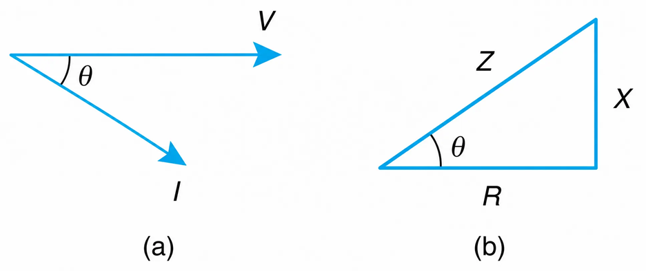
Figure 1-33 Power-factor angle. (a) Voltage–current phasors. (b) Inductive impedance diagram.

When the current is lagging the voltage (inductive loads), the power factor is said to be lagging, and when the current is leading the voltage (capacitive loads), the power factor is said to be leading. The range of the power factor is between 40 and 100%.

A low or a poor power factor is a characteristic of digital communication transmitters, small motors, partially loaded large motors, welders, and the like. A 100% power factor is, of course, associated with electric heaters.

Mathematically, the power factor could be given by any of the following relations:

$$\cos\theta=\frac{R}{|Z|} \ \ \ \ \ (1.91)$$

where R and Z are, respectively, the load’s resistance and the magnitude of the impedance.

Also,

$$\cos\theta=\frac{P}{S} \ \ \ \ \ (1.92)$$

where P and S are, respectively, the average and apparent power of the load.

The previous relationship can be also written as follows:

$$\cos\theta=\frac{VI_P}{\sqrt{(VI_P)^2+(VI_r)^2}} \ \ \ \ \ (1.93)$$

where V is the load’s voltage and I_P and I_r are, respectively, the magnitudes of real and reactive components of the load’s current (I).

$$I=I_P+I_r \ \ \ \ \ (1.94)$$

For example, when

$$I = 10\angle -37^\circ\ \text{A}$$

Then

$$I_P = 10\cos 37^\circ = 8\ \text{A}$$

And

$$I_r = 10\sin(-37^\circ) = 6\ \text{A}$$

The power factor calculated from the previous expressions is termed the apparent power factor. The actual power factor is slightly lower than that because of the system’s harmonics.

When the harmonic component of the current (I_h) is known, the actual power factor is given by

$$\cos\theta=\frac{VI_P}{\sqrt{(VI_P)^2+(VI_r)^2+(VI_h)^2}} \ \ \ \ \ (1.95)$$

Example 1-11

The apparent power factor of a 208 V, 5 kW load is 0.75 lagging, and its harmonic current is 15% to that of the fundamental. Calculate the actual power factor.

Solution

$$I=\frac{5000}{(208)(0.75)}=32.05\angle -41.4^\circ\ \text{A}$$

$$I=24.01-j21.20$$

And

$$I_h = 0.15(32.05)$$

$$I_h = 4.81\ \text{A}$$

Substituting in Equation (1.95), we obtain

$$\cos\theta=\frac{208(24.01)}{\sqrt{\left(208(24.01)\right)^2+\left(208(21.20)\right)^2+\left(208(4.81)\right)^2}}=0.74\ \text{lagging}$$

In this case, there is no substantial difference between the actual and apparent power factor.

Effects of the Power Factor

From Equation (1.80), the current is given by

$$I=\frac{P}{V\cos\theta} \ \ \ \ \ (1.96)$$

Say,

$$\frac{P}{V} = 100$$

Then,

$$\text{For }\theta = 60^\circ,\ \cos 60^\circ = 0.5,\ I = 200\ \text{A}$$

$$\text{For }\theta = 0^\circ,\ \cos 0^\circ = 1,\ \text{and}\ I = 100\ \text{A}$$

That is, the power factor controls the current to a load. The lower the power factor, the higher the current. The technical and economical disadvantages of the low power factor (higher current) are the following:

1.     Higher generator (I²R)

2.     Larger generator

(The generators are purchased or rated in volt x amps.)

3.     Higher cable losses (I²R)

4.     Larger diameter of cable

(The larger the diameter of a cable, the more current it can carry.)

5.     Larger transformer losses (I²R)

6.     Larger size of transformer

(The transformers are purchased or rated in volt x amps.)

7.     The lower the voltage across the load (V_L)

$$V_L=V_{\text{source}}-IZ \ \ \ \ \ (1.97)$$

where Z is the impedance of the source.

The lower the load voltage, the lower the torque (T).  Also, the lower the voltage, the lower the light output of the lighting fixtures. It is for the above reasons that the utilities penalize customers who operate at low power factors.

In general, it can be said that the power factor is the effectiveness of the current, just as in a mechanical system, the cosine of the angle between the force and the direction of displacement is a measure of the effectiveness of the force.

Similarly, a person expends less calories by walking on level ground than by walking uphill because the phase angle between the force (weight) and the direction (horizontal) is 90° degrees. Energy is equal to the force times its displacement times the cosine of the angle between the force and its displacement.

Calculation of Penalty

The utilities use one of the following two techniques to penalize consumers for poor power factor.

• They charge for kVA registered regardless of phase angle θ. Since the kVA depends on θ, there is always an additional charge for θ larger than zero degrees.
• They charge for kVA registered in conjunction with θ above a given magnitude (usually 26°) as follows:

They measure the month’s apparent (S) and average power (P). Then based on their minimum power-factor requirements ($cos\theta_{m}$), they compare the following:

$$S(\cos\theta_m)\ \text{and}\ P$$

For billing purposes, they select the largest of the two. The kW penalty is the difference of the two. For example, assume that a utility’s minimum power factor is 90%, while a plant operates at 0.80 Pf and draws 100 kVA and 80 kW. Then the penalty is calculated as follows:

$$S\cos\theta_m = 100(0.9) = 90\ \text{kW}$$

The customer is charged an extra

$$90 - 80 = 10\ \text{kW}$$

The term $Scos\theta_{m}$ is often referred to as the corrected power in kW. Its cost depends on the monthly charges/kW. The minimum power-factor requirement is a commercial term chosen by the utility.

Power-Factor Correction using Capacitors

Since the current through a capacitor leads its voltage and that through an inductive load lags its corresponding voltage, the parallel hook-up of a capacitor to such a load will reduce the current drawn from the utility.

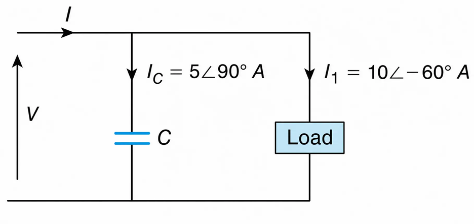
Figure. 1-34 Usage of a capacitor to reduce the line current.

The current supplied by the source is given by

$$I = I_c + I_1$$

$$= 5\angle 90^\circ + 10\angle -60^\circ$$

$$= 6.20\angle -36.2^\circ\ \text{A}$$

That is, by connecting the capacitor in parallel to the load, the current supplied by the utility was reduced from 10 A to 6.20 A and its phase angle was also reduced from 60 degrees to 36.2 degrees. The power factor of the load, however, does not change. A similar conclusion can be drawn by adding up the current phasors graphically.

Consider Figure 1-35.

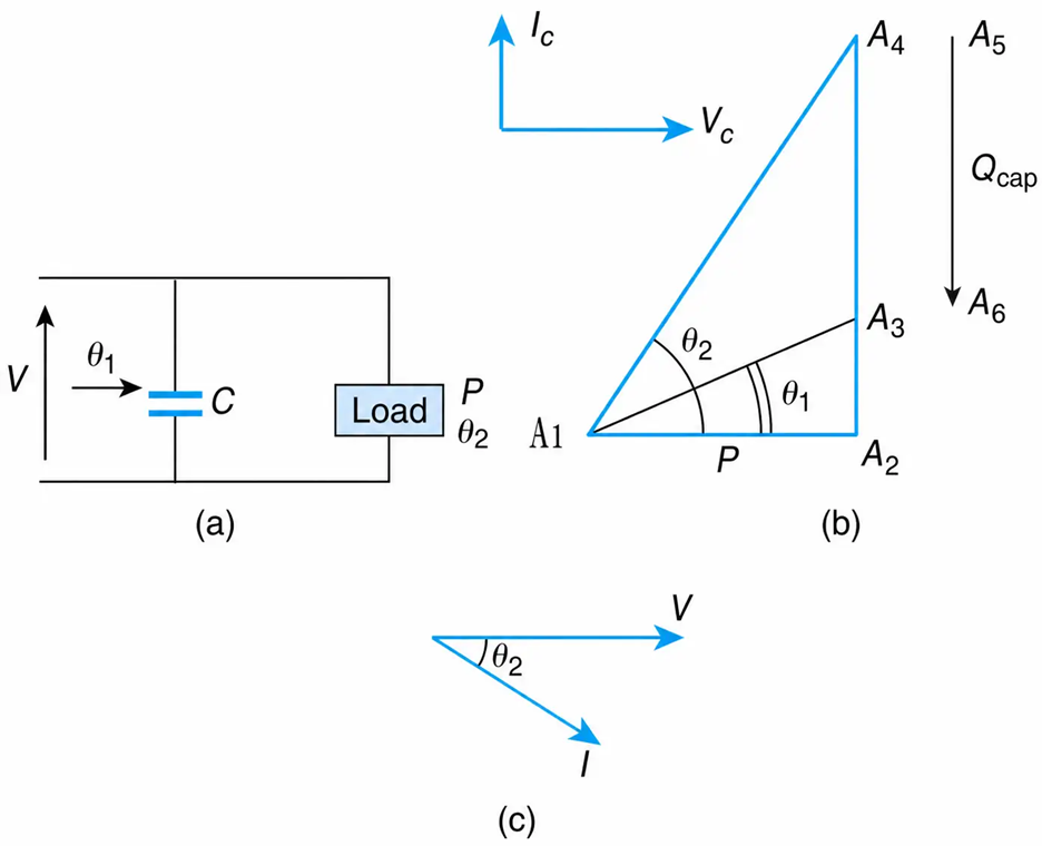
Figure. 1-35 Power-factor correction. (a) Circuit. (b) Power representation. (c) Voltage-current waveforms.

The powers of an inductive load are represented graphically by the triangle A₁A₂A₄ , which is referred to as the load’s power triangle. The voltage-current phasor of a capacitor and its corresponding power representation A₅A₆ (S = Q and P = 0 ) are shown in Figure 1-35(b).

In order to increase the power factor from $cos\theta_{2}$ to $cos\theta_{1}$ , the reactive power represented by the length A₃A₄ must be removed by connecting a capacitor in parallel to the load.

From the triangle,

$$A_3A_4 = A_2A_4 - A_2A_3$$

Or

$$= P\tan\theta_2 - P\tan\theta_1$$

When P is kW and A₃A₄ is in capacitive kVAR (Q), then

$$Q=P\left(\tan\theta_2-\tan\theta_1\right) \ \ \ \ \ (1.98)$$

Equation (1.98) can be used to select the capacitor requirements to change θ₂ to θ₁.

Example 1-12

Refer to circuit Figure 1-36. Determine the circuit’s

a. Impedance.

b. Inductance

c. Current.

d. Power factor.

e. Average power supplied.

f. Complex, apparent, and reactive power.

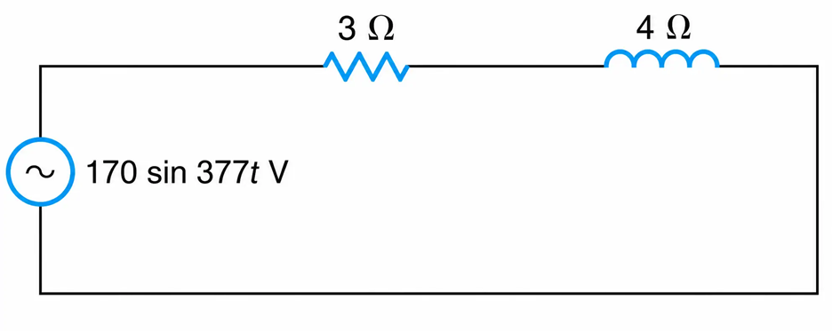
Figure 1-36 RL Series Circuit

Solution

a.     The impedance is

$$Z = R + jX$$

$$= 3 + j4 = 5\angle 53.1^\circ\ \Omega$$

b.    The inductive reactance is

$$X = 4\ \Omega$$

$$\omega L = 4\ \Omega$$

$$L = \frac{4}{377} = 10.61\ \text{mH}$$

c.     The current is

$$I=\frac{V}{Z}$$

$$=\frac{170\sqrt{2}}{3+j4}=24.04\angle -53.1^\circ\ \text{A}$$

d.    The power factor is

$$\cos\theta = \cos 53.1^\circ$$

$$\cos\theta = 0.60\ \text{lagging}$$

e.     The average power is

$$P = VI\cos\theta = \frac{170}{\sqrt{2}}(24.04)\cos 53.1^\circ = 1734.0\ \text{W}$$

Or

$$P = I^2R = (24.04)^2(3) = 1734.0\ \text{W}$$

f.      The complex power is

$$S = VI^{*} = \frac{170}{\sqrt{2}}\,24.04\angle 53.1^\circ = 2890.0\angle 53.1^\circ\ \text{VA}$$

and the apparent power is

$$S = |VI|$$

$$S = 2890.0\ \text{VA}$$

The reactive power is

$$Q = VI\sin\theta$$

$$Q = \frac{170}{\sqrt{2}}(24.04)\sin 53.1^\circ$$

$$Q = 2312.00\ \text{VARs}$$

Or

$$Q = I^2X$$

$$Q = (24.04)^2(4)$$

$$Q = 2312.00\ \text{VARs}$$

Example 1-13

A 480 V, 40 kW load operates at a Pf of 80%. Determine:

a.     The utility’s penalty per year when the charges for the power factor are less than 100% are $11/kW/month.

b.    The size and cost of the capacitor bank improve the power factor to 100% when the purchasing cost of the capacitor is $40/kVAR.

Solution

a.     $$S = \frac{P}{\cos\theta} = \frac{40}{0.8} = 50\ \text{kVA}$$

            $$\text{Penalty} = 50 - 40 = 10(1) = 10\ \text{kW}$$

Its cost(C)

$$C = 10(11)(12) = \$1320/\text{year}$$

b.    The size of the capacitor bank is

$$Q = P\left(\tan\theta_2 - \tan\theta_1\right)$$

$$Q = 40\left(\tan 36.9^\circ - \tan 0^\circ\right) = 30\ \text{kVAR}$$

Its cost(C) is

$$C = 30(40) = \$1200.00$$

That is, the payback period is less than one year.

Example 1-14

A 230 V, 60 Hz voltage source supplies rated power to three loads whose characteristics are shown in Figure 1-37(a). Assuming that each load’s efficiency is 90%, determine:

a.     The overall power factor of the system.

b.    The magnitude of the current drawn from the voltage source.

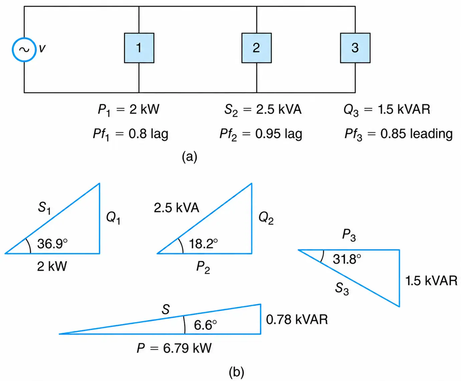
Figure. 1-37 Characteristics of Different Loads

Solution

a.     The individual power triangles are constructed from the given data. The input overall power triangle can be obtained graphically from the individual power triangles (see Figure 1-37(b)) or mathematically as follows. The input real power is

$$P = \frac{1}{\eta}\left(P_1 + P_2 + P_3\right)$$

Where $\eta$ is the efficiency (output power/input power) of each load. Substituting the equivalent equations for P₂ and P₃, we obtain

$$P=\frac{1}{\eta}\left(P_1+S_2\cos\theta_2+\frac{Q_3}{\tan\theta_3}\right)$$

$$P=\frac{1}{0.9}\left[2+2.5(0.95)+\frac{1.5}{\tan 31.8^\circ}\right]$$

$$P=7.55\ \text{kW}$$

The input reactive power is

$$Q=\frac{1}{\eta}\left(Q_1+Q_2-Q_3\right)$$

$$Q=\frac{1}{\eta}\left(P_1\tan\theta_1+S_2\sin\theta_2-Q_3\right)$$

$$Q=\frac{1}{0.9}\left(2\tan36.9^\circ+2.5\sin18.2^\circ-1.5\right)$$

$$Q=0.87\ \text{kVAR}$$

The complex power is

$$S = P + jQ$$

$$= 7.55 + j0.87 = 7.6\angle 6.6^\circ\ \text{kVA}$$

The power factor is

$$\cos(6.6^\circ) = 0.99\ \text{lagging}$$

b.    The magnitude of the current is

$$I=\frac{|S|}{V}=\frac{7600}{230}=33.0\ \text{A}$$