Single-Phase Transformer Operation and Equivalent Circuit
As shown in Figure 2-3, single-phase transformers usually have one input and one output winding, often referred to as the transformer’s primary and secondary windings. These windings are not electrically connected but are magnetically coupled. The primary winding draws energy from a voltage source, whereas the secondary winding delivers energy to a load.
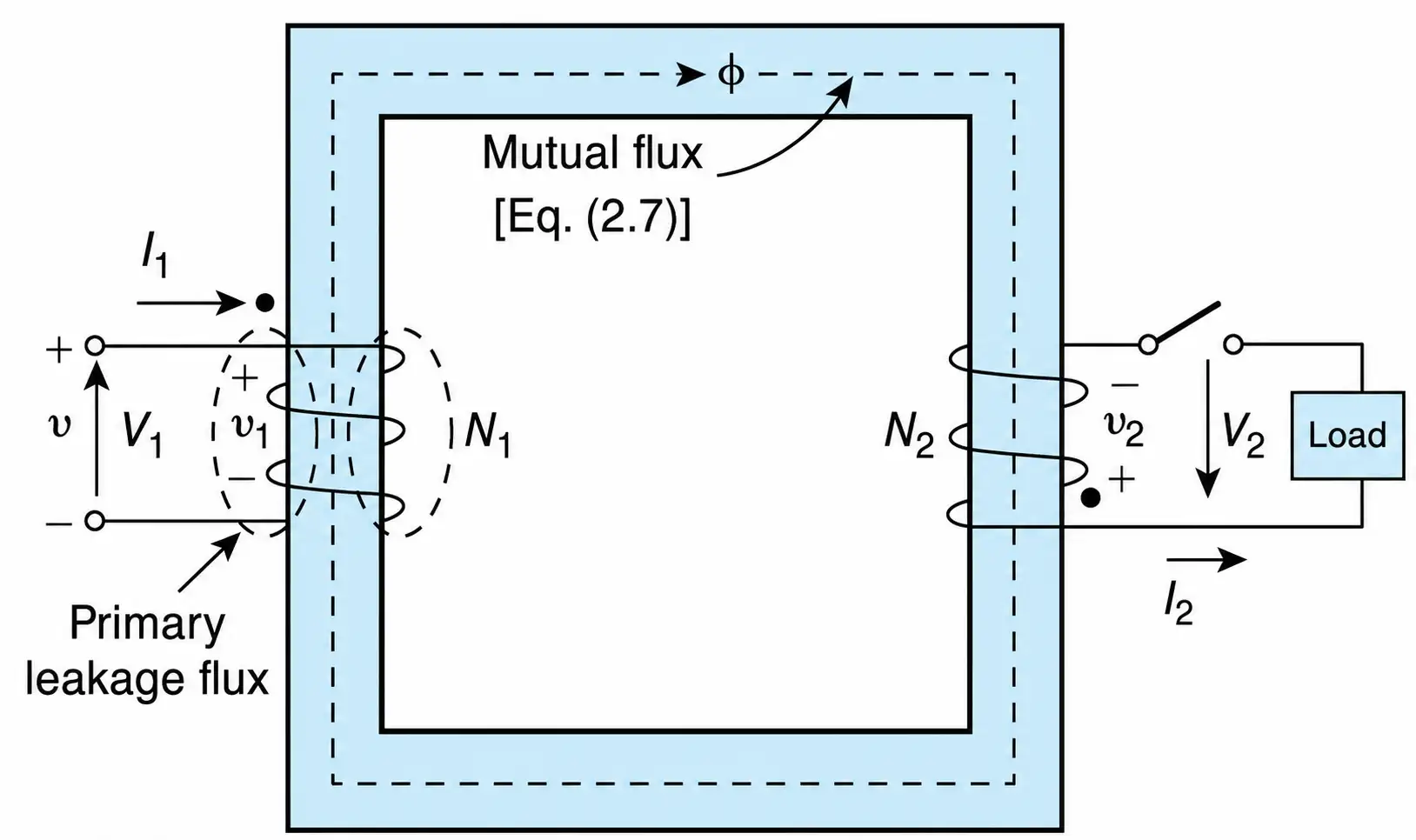
Figure 2-3 Single-phase transformer.
Transformers are not power amplifiers. For all practical purposes, the apparent input power ($|S|$) to a transformer’s primary winding is equal to the apparent power delivered to the load by its secondary winding. In other words, the volt-amperes of the primary winding (V1I1) are approximately equal to the volt-amperes of the secondary winding (V1I2) . Mathematically,
$$|S|=V_1I_1\approx V_2I_2 \ \ \ \ \ (2.1)$$
In actual cases—because of transformer losses—the volt-amperes delivered to a load by a transformer are slightly less than the volt-amperes drawn from the voltage source.
Principle of Operation
The operation of single-phase transformers (and all other transformers) is based on the principle of induction. According to this principle, a voltage is induced in a winding when the winding’s flux linkages (λ) change as a function of time. The instantaneous value of the flux linkages is defined as
$$\lambda=N\phi \ \ \ \ \ (2.2)$$
where N and $\phi$ are, respectively, the coil’s number of turns and the instantaneous value of the flux per turn. Alternatively,
$$\lambda=Li \ \ \ \ \ (2.3)$$
where L and i are, respectively, the coil’s inductance and instantaneous current.
According to Faraday’s law, the instantaneous value of the induced voltage (v) is given by
$$v=-\frac{d\lambda}{dt} \ \ \ \ \ (2.4)$$
Or
$$v=-\frac{d}{dt}(N\phi) \ \ \ \ \ (2.5)$$
The minus sign in the equations signifies that the voltage induced opposes the supply voltage. This, however, is not necessary because the application of KVL in the corresponding loop will yield the proper sign. Furthermore, the voltage has a meaning when you identify the two terminals across which the voltage is measured. The induction principle can also be explained by using the following simple everyday logic.
The flux lines of the primary current disturb—pass through—the secondary coil that, because “action is equal and opposite to reaction,” produces its own current and flux in order to oppose the disturbance. This current and/or flux is associated with the voltage developed. The voltage developed is also referred to as the voltage produced, induced, or generated.
From Equation (2.5):
$$v=-N\frac{d\phi}{dt} \ \ \ \ \ (2.6)$$
The negative sign in the equation signifies that the polarity of the induced voltage opposes the change that produced it. This reaction is a natural one for magnetically coupled coils and follows the principle commonly known as Lenz’s law.
As shown in Figure 2-3, the polarity of the induced voltages is usually identified by the dot symbol.
Equation (2.6) is a basic law of electromagnetism and one of the most important mathematical relationships of electrical engineering. It governs the operation of motors and generators, and it demonstrates the coexistence of, and the quantitative relationship between, electric and magnetic fields.
The flux within the structure of the transformer changes because it is produced by the alternating voltage supplied to the transformer’s input winding.
As Equation (2.6) makes clear, for sinusoidal input voltages the flux is at a maximum when the voltage is at the zero point of its cycle. The flux and the voltage phasors must be 90° out of phase with each other. Typical voltage and flux waveforms for a transformer are shown in Figure 2-4.
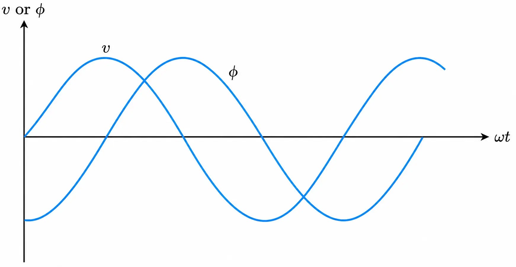
Figure 2-4 Voltage and flux waveforms in a single-phase transformer.
Equation (2.7) relates the induced voltage to the magnetic flux and is of fundamental importance to the understanding of transformers and electric machines.
$$V=4.44Nf\phi_m \ \ \ \ \ (2.7)$$
where V is the rms value of the input voltage, f its frequency of oscillation in hertz, and $\phi_m$ the maximum value of the flux within the magnetic material in Weber.
Thus, the rms value of the voltage induced in the secondary winding of the transformer, or in any other coil wound on the same core, will be given by Equation (2.7). In each case, the appropriate number of turns must be used.
Equation (2.7) is called the fundamental transformer equation, and it is often used in laboratories to calculate the flux level within any shape—toroidal, rectangular, and so on—of magnetic circuit. This equation gives accurate results only if the leakage impedance of the coil is negligible.
The flux produced by the primary winding is divided into two parts: leakage flux and mutual flux. Leakage flux links only the windings of the primary coil and is associated with the transformer leakage impedance. Mutual flux links the windings of the primary and secondary coils and is associated with the magnetizing impedance of the transformer.
Ideal Transformer Relationships
In this section we derive general equations that relate the parameters of the primary winding to the parameters of the secondary winding. We will consider only ideal transformers in order to provide the basis for analysis of nonideal transformers.
An ideal transformer has zero core loss, no leakage flux, and negligible winding resistances. Refer to Figure 2-5. Using the induction principle, we have
$$v_1=-N_1\frac{d\phi}{dt} \ \ \ \ \ (2.8)$$
$$v_2=-N_2\frac{d\phi}{dt} \ \ \ \ \ (2.9)$$

Figure 2.5 An illustration of the concept of voltage induced. Only the mutual flux is shown.
$$\upsilon_2=\upsilon_1\frac{N_2}{N_1} \ \ \ \ \ (2.10)$$
Under the assumed ideal conditions, the induced voltages (v1 , v2) are equal to their corresponding terminal voltages. Then using rms values, we obtain
$$V_2=V_1\frac{N_2}{N_1} \ \ \ \ \ (2.11)$$
That is, voltages of different magnitudes can be obtained by winding coils with different numbers of turns around a magnetic circuit. The effective flux ($\phi$) within the magnetic material is dependent on the applied voltage and is essentially independent of the flux of the output current. Thus, under ideal conditions, the voltage induced in the output winding is independent of the load current.
Figure 2-6 shows a schematic of a two-winding transformer, its magnetic equivalent circuit, and its ideal electrical equivalent circuit.
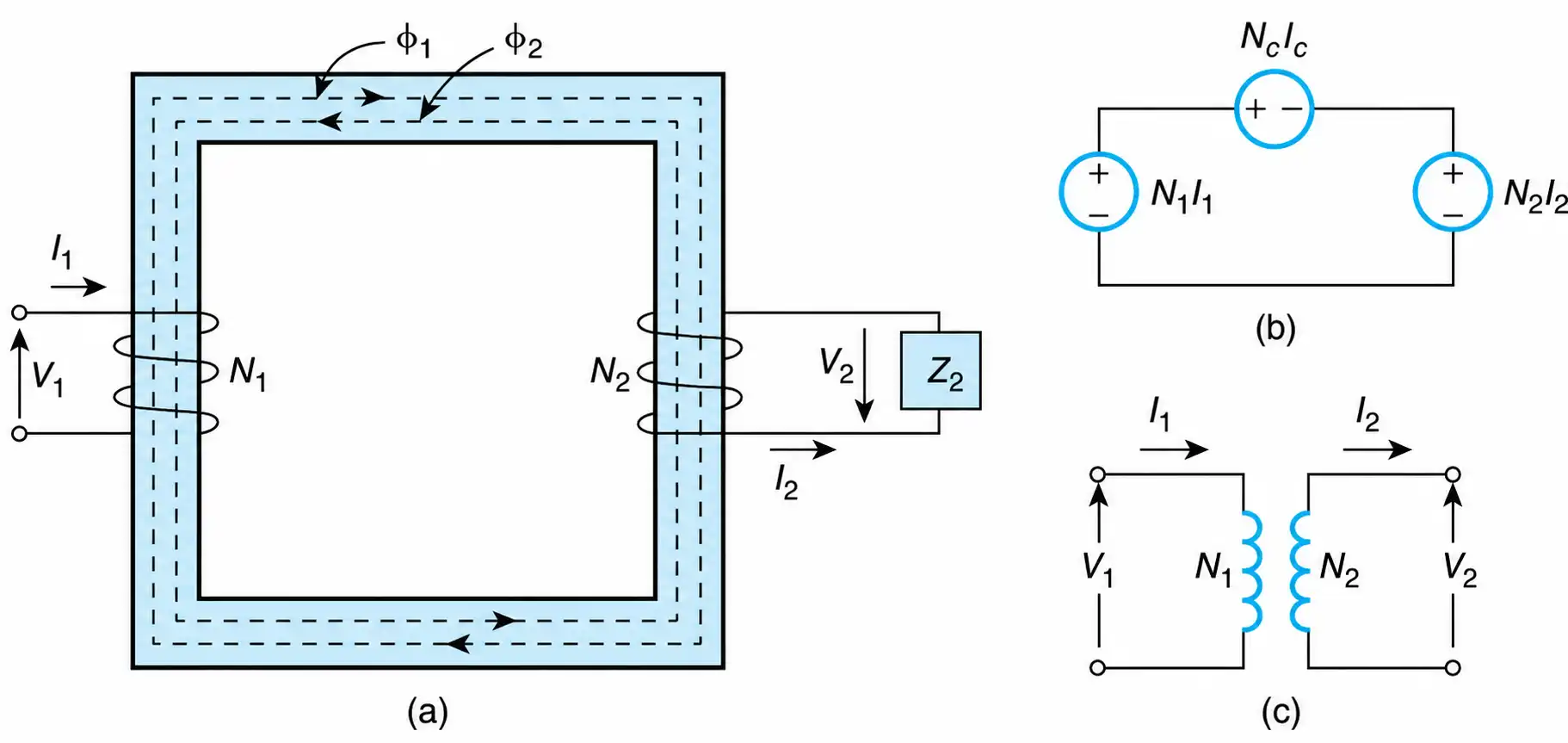
Figure 2-6 An ideal transformer. (a) Physical representation. (b) Equivalent magnetic circuit. (c) Equivalent electrical circuit.
$$\sum (NI)_{\text{loop}}=0 \ \ \ \ \ (2.12)$$
That is, the sum of the magnetic potentials or ampere-turns within a closed magnetic circuit is equal to zero. In mathematical symbols,
$$(N_1I_1)_{\text{input}}-(N_cI_c)_{\text{core}}-(N_2I_2)_{\text{output}}=0 \ \ \ \ \ (2.13)$$
The magnetic potential (NcIc)core is the amount of magnetomotive force (mmf) required to magnetize the core of the transformer. For an ideal transformer ($\mu =\infty$) , this mmf is equal to zero. That is,
$$(N_c I_c)_{\text{core}} = 0$$
Thus, from Equation (2.13), we have
$$I_2=I_1\frac{N_1}{N_2} \ \ \ \ \ (2.14)$$
From Ohm’s law, we obtain
$$Z_1=\frac{V_1}{I_1} \ \ \ \ \ (2.15)$$
And
$$Z_2=\frac{V_2}{I_2} \ \ \ \ \ (2.16)$$
where Z1 and Z2 are not the winding impedances, but the impedances as seen from the terminals of winding 1 and winding 2, respectively.
From Equations (2.11), (2.14), (2.15), and (2.16), we obtain the impedance transformation property of transformers. That is,
$$Z_1=Z_2\left(\frac{N_1}{N_2}\right)^2 \ \ \ \ \ (2.17)$$
It should be emphasized that Equations (2.11), (2.14), and (2.17) are applicable only to ideal transformers. An ideal transformer is represented by the equivalent circuit shown in Figure. 2-6(c).
Example 2-1
The 5 kVA, 480-120 V, single-phase transformer shown in Figure. 2-7 delivers rated current to a 120 volt load. Neglecting losses, determine the transformer currents and the supply voltage.
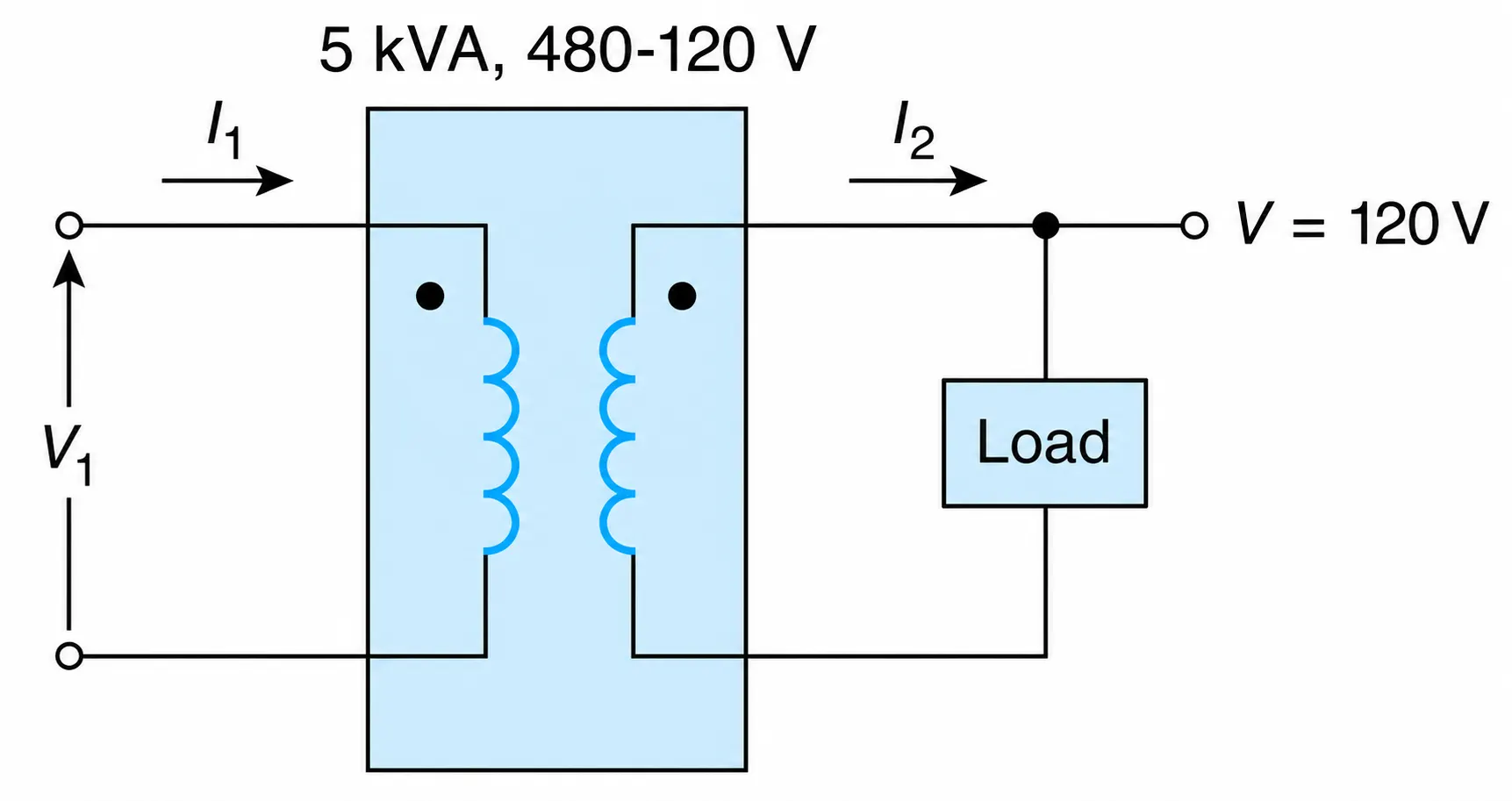
Figure 2-7 5 kVA, 480-120 V, single-phase transformer
Solution
The magnitude of the current through the secondary winding is
$$I_2 = \frac{|S|}{V} = \frac{5000}{120} = 41.67A$$
The windings turns ratio is given by the ratio of the windings voltages:
$$\frac{N_2}{N_1} = \frac{V_2}{V_1} = \frac{120}{480} = \frac{1}{4}$$
From Equation (2.14), the magnitude of the current through the primary winding is
$$I_1 = \frac{1}{4}(41.67) = 10.42A$$
The primary voltage is given by the rating of the transformer. That is,
$$V_1 = 480 \ \text{volts}$$
In an actual transformer, the primary voltage and current would be slightly higher than calculated here because of the effect of the transformer’s impedances.
Derivation of the Equivalent Circuit
The analysis of transformers is greatly simplified by using a model, called the equivalent circuit. Figure 2-8 shows various forms of the equivalent circuit of a single-phase transformer. Figure 2-8(a) is the schematic of a single-phase transformer, and its approximate equivalent circuit is shown in Figure. 2-8(b).
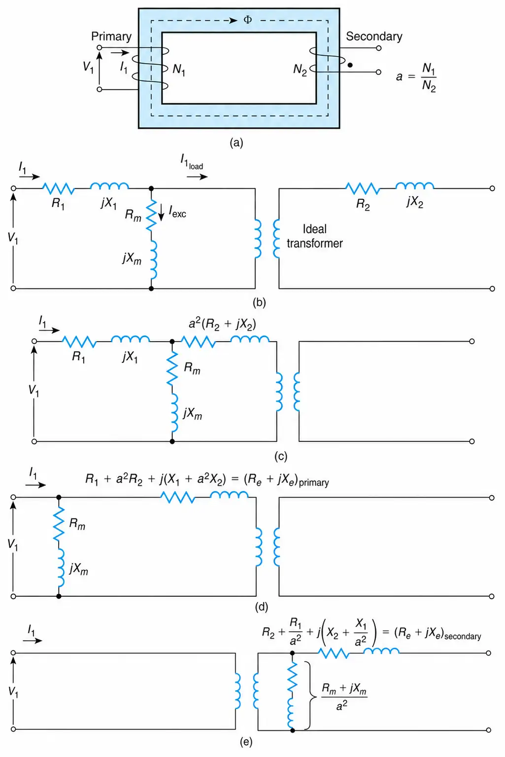
Figure 2-8 Various forms of the equivalent circuit of a single-phase transformer. (a) Elementary schematic. (b) Individual winding impedances and the magnetizing impedance. (c) All impedances transferred to the primary. (d) An approximation of part (b). (e) All impedances referred or transferred to the secondary.
The resistance R1 and the X1 reactance represent the copper losses and the leakage flux of the primary winding, respectively. Similarly, the resistance R2 and the reactance X2 represent the copper losses and the leakage flux of the secondary winding, respectively. Then $R_{1}+jX_{1}$ and $R_{1}+jX_{1}$ represent the impedances of the primary and secondary windings, respectively. These impedances are often referred to as leakage impedances.
The winding with the higher voltage rating has higher leakage impedance than the winding with the lower voltage rating. Rm represents the core-loss equivalent resistance, and $X_{m}$ represents the magnetizing reactance of the transformer. Usually, the magnetizing impedance is represented by a core resistance ($R_{c}$) in parallel with a magnetizing reactance $X_{\phi}$ [see Figure. 2-8(c)].
The resistance $R_{m}$ represents the so-called magnetizing or core losses, that is, eddy-current and hysteresis losses.
Typical core losses are given in Tables 2-1 and 2-2. Scientists and manufacturers constantly develop higher quality material and thus tomorrow’s transformers will have lower losses.
Table 2-1 Parameters of 4160–480/277 V, Dry-Type Transformers with Copper Windings
|
Rating (kVA) |
Resistance in Ohms at 70°C (HV) |
Resistance in Ohms at 70°C (LV) |
Exciting Current (%) |
Core Losses (kW) |
Copper Losses (kW) |
Efficiency at Full Load (%) |
Impedance (%) |
|
500 |
2.90 |
0.011 |
1.50 |
1.2 |
7.6 |
98.3 |
5.5 |
|
1000 |
1.09 |
0.004 |
1.12 |
3.8 |
13.1 |
98.3 |
5.9 |
|
1500 |
0.75 |
0.003 |
0.70 |
4.0 |
20.0 |
98.4 |
6.1 |
|
2000 |
0.48 |
0.016 |
0.65 |
4.8 |
23.0 |
98.6 |
6.5 |
Table 2-2 Parameters of a 15/20/22.4 MVA, 60–4.16/2.4 kV, Liquid-Type Transformer with Copper Windings
|
Exciting Current in Percent |
Core Loss in kW |
Copper Loss in kW |
Impedance in Percent |
|
0.41 |
15.0 |
65 |
7.0 |
In Figure. 2-8(c), the leakage impedance of the secondary winding is transferred to the primary.
In Figure. 2-8(d), the magnetizing impedance is relocated to the input terminals of the transformer. This equivalent circuit, though approximate, simplifies the calculations.
In Figure. 2-8(e), all impedances shown in Figure. 2-8(d) are transferred to the secondary winding.
The leakage impedance is calculated from the “short-circuit test” data, and the magnetizing impedance is calculated from the “open-circuit test” data.
Short-Circuit Test
The short-circuit test (also referred to as the impedance or copper-loss test) can be done on either side of the transformer. The input power ($P_{z}$) , the applied voltage ($V_{z}$) , and the input current ($I_{z}$) are measured in one winding, while the other winding, as shown in Figure. 2-9, is short-circuited. The objective of this test is to find the power loss in the windings of the transformer and the equivalent winding impedances under rated conditions. The winding power losses affect the efficiency of the transformer, and the leakage impedance affects the short-circuit current and the output voltage of the transformer. For this reason, rated current is used in this test. Thus,
$$I_z = I_{\text{rated}}$$
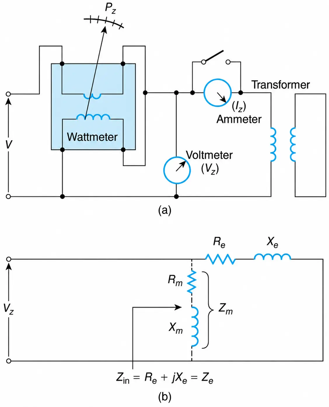
Figure 2-9 Short-circuit test. (a) Laboratory connection schematic. (b) Equivalent circuit. (Notice that the magnetizing impedance Zm is considered infinite.)
In practice, a near rated value is used, and then proper adjustments are made to related calculations so that the parameters obtained represent the transformer at nominal operating condition.
The voltage $V_{z}$ is only a small percentage of the rated voltage and is sufficient to circulate rated current in the windings of the transformer. Usually,
$$V_z=(2\%\rightarrow12\%)V_{\text{rated}}$$
As a result, the transformer is magnetized at a relatively low flux density, as shown in Figure. 2-11. In performing this test, the magnetizing impedance is assumed to be open because, in relative terms, it is very large.
Neglecting the losses of the measuring instruments, we have
$$R_e=\frac{P_z}{I_z^2}\,\text{ohms} \ \ \ \ \ (2.18)$$
$$|Z_e|=\frac{V_z}{I_z}\,\text{ohms} \ \ \ \ \ (2.19)$$
$$X_e=\sqrt{Z_e^2-R_e^2}\,\text{ohms} \ \ \ \ \ (2.20)$$
This test does not give the individual winding impedances, but rather the combined impedances of primary and secondary windings. The subscript e is used to indicate that the short-circuit test gives the equivalent transformer leakage impedance, or the combination of the winding impedances as seen from one of the transformer windings.
The winding parameters as calculated from Equations (2.18), (2.19), and (2.20) are said to be referred to the side of the transformer where the instruments were placed. However, you can easily transfer this impedance to the other side of the transformer by multiplying it by the turns ratio squared. The turns ratio used must be the one seen from the side of the transformer to which this impedance is to be referred.
Open-Circuit Test
The open-circuit test (also referred to as the core-loss test, the magnetization test, the excitation test, the iron-loss test, or the no-load test) furnishes the core loss and the magnetizing impedance under rated conditions. It is usually done on the side of the transformer that has the lower rated voltage.
In conducting this test, the equivalent leakage impedance of the transformer is considered negligible because it is, relatively speaking, very small. The excitation power ($P_{exc}$) , the excitation current ($I_{exc}$) , and the excitation voltage ($V_{exc}$) are measured in one winding, as shown in Figure. 2-10(a), while the other winding is open-circuited. Neglecting the losses of the measuring meters, we have
$$R_m=\frac{P_{\text{exc}}}{I_{\text{exc}}^2}\,\text{ohms} \ \ \ \ \ (2.21)$$
$$|Z_m|=\frac{V_{\text{exc}}}{I_{\text{exc}}}\,\text{ohms} \ \ \ \ \ (2.22)$$
And
$$X_m=\sqrt{Z_m^2-R_m^2}\,\text{ohms} \ \ \ \ \ (2.23)$$
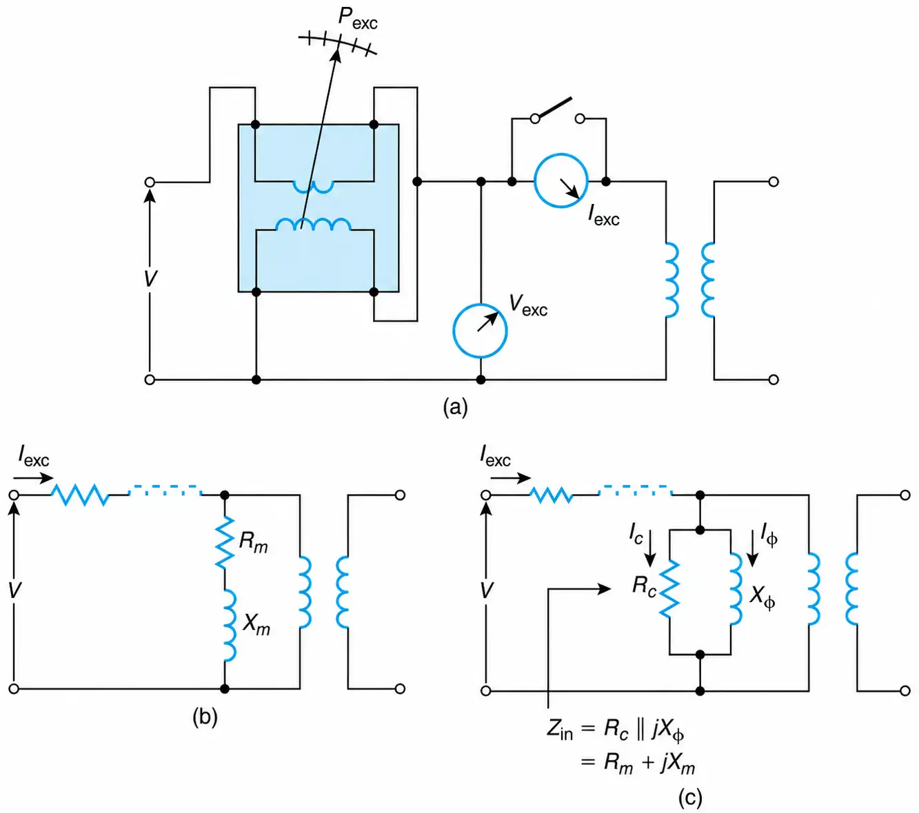
Figure 2-10 Open-circuit test. (a) Laboratory connection schematic. (b) Series representation of the magnetizing impedance (notice that R1+JX1 are considered negligible). (c) Parallel representation of the magnetizing impedance.
The excitation current is a small percentage of the transformer’s nominal current. Usually,
$$I_{\text{exc}}=(3\%\rightarrow10\%)I_{\text{rated}}$$
In order to obtain the core loss that corresponds to rated conditions, the flux on open-circuit test must be equal to the flux within the transformer when the transformer delivers rated current. This is insured, as can be seen from Equation (2.7), when the excitation voltage is equal to the rated voltage. That is,
$$V_{\text{exc}} = V_{\text{rated}}$$
Thus, as shown in Figure. 2-11, on an open-circuit test the transformer is energized at approximately the same flux level as under normal operating conditions.
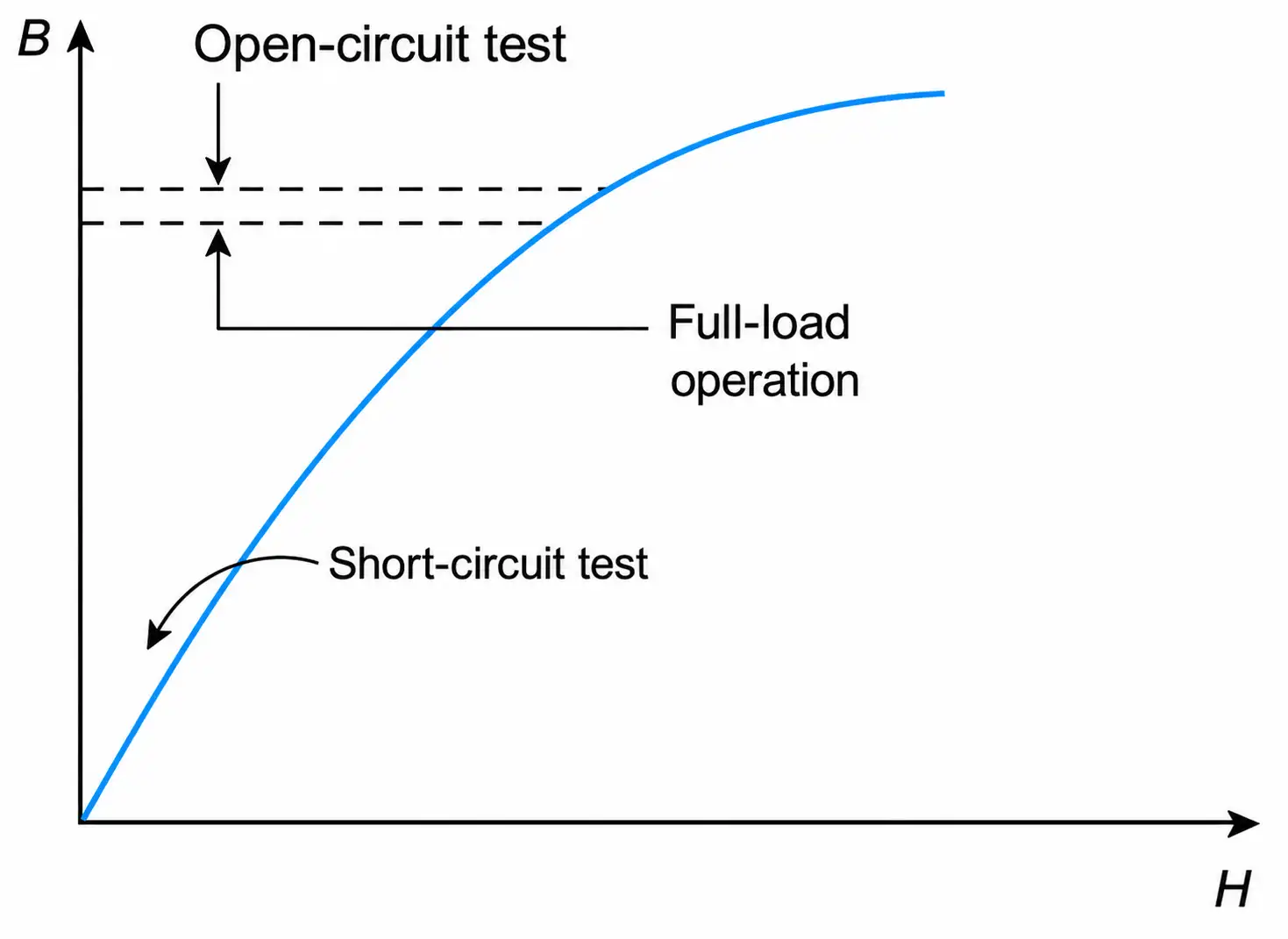
Figure 2-11 B-H curve, showing the relative magnetization levels for a transformer during a short-circuit test, open-circuit test, and under full-load operating conditions.
The transformer’s magnetizing parameters as calculated from Equations (2.21), (2.22), and (2.23) are as seen from the side of the transformer where the instruments were placed. It can be easily transferred or referred to the other side by using the impedance transformation property of ideal transformers.
When the core loss is measured at other than the operating voltage, then the actual copper losses can be calculated by considering them as being proportional to the square of the applied voltage.
In the open-circuit test, both primary and secondary voltages are customarily recorded. This gives the effective turns ratio of the transformer, which might be slightly different from the ratio specified on its nameplate.
The series representation of the magnetizing impedance can be represented by its equivalent parallel impedance, as shown in Figure. 2-10(c). The equations that relate the components of the series equivalent impedance to those of the equivalent parallel impedance, Equations (1.179) and (1.180), are repeated here for convenience:
$$R_c=\frac{R_m^2+X_m^2}{R_m} \ \ \ \ \ (2.24)$$
$$X_{\phi}=\frac{R_m^2+X_m^2}{X_m} \ \ \ \ \ (2.25)$$
The series impedance representation tends to simplify the calculations, but the parallel representation reveals more about the magnetization process and thus is more common. For example, an inspection of the parallel impedance representation gives the core losses $P_{\text{exc}} = \frac{V^2}{R_c}$ and the components of the exciting current $I_{\phi} = \frac{V}{jX_{\phi}}, I_c = \frac{V}{R_c}$. The core or open-circuit losses are caused by eddy currents and hysteresis losses. Typical winding and iron losses for a 5 kVA single-phase transformer as a function of load current are shown in Figure. 2-12.
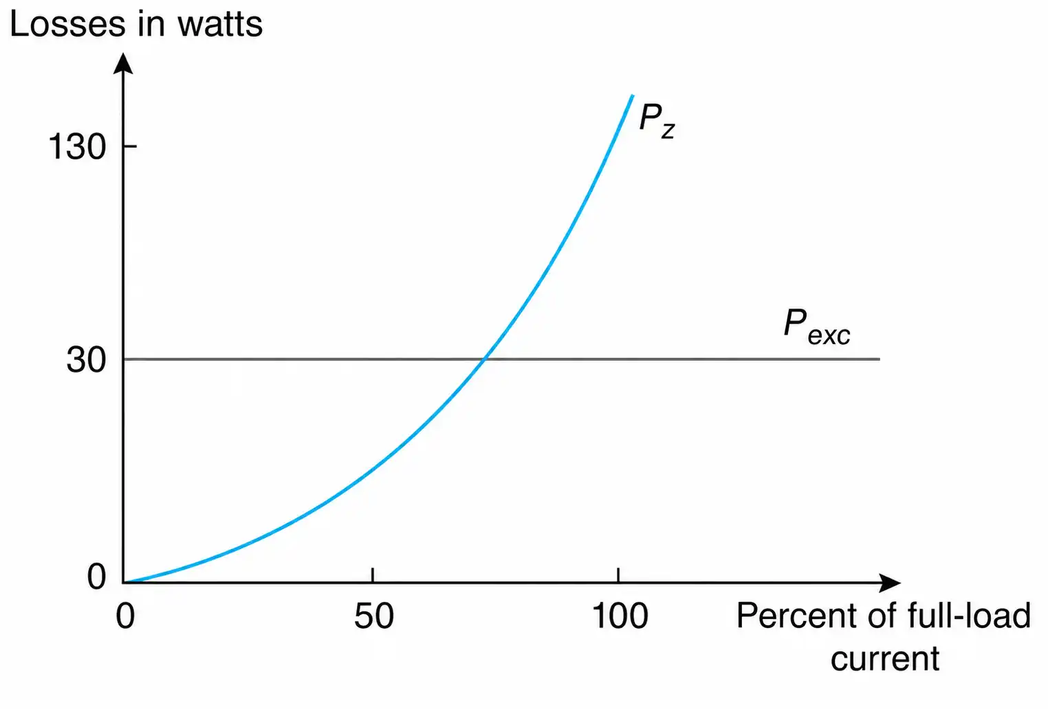
Figure 2-12 Typical winding and iron losses as a function of load current for a single-phase transformer (5 kVA, 480–120 V).
In concluding this section on transformer tests, it must be emphasized that Ze is the input impedance of the transformer when its secondary is shorted, and Zm is the input impedance of the transformer when its secondary is open-circuited. These statements are, of course, approximate because of the underlying assumptions.
Example 2-2
The following results were obtained from testing a 10 kVA, 480-120 V, single-phase transformer.
|
Test |
Voltage in Volts |
Current in Amperes |
Power in Watts |
|
Open-circuit |
120 |
2.5 |
60 |
|
Short-circuit |
26 |
20.83 |
200 |
Determine:
a. The equivalent leakage impedance of the transformer windings referred to the high-voltage (HV) and low-voltage (LV) winding.
b. The series and parallel components of the magnetizing branch referred to the LV winding.
c. The equivalent circuit of the transformer referred to the HV winding.
Solution
a. The rated current of the transformer through the primary and secondary windings is:
$$I_H = \frac{|S|}{V} = \frac{10000}{480} = 20.83A$$
$$I_L = \frac{10000}{120} = 83.33A$$
By comparing the above with the given test data, it is clear that the short-circuit test was done on the HV winding.
Thus,
$$R_{eH} = \frac{P_z}{I_z^2} = \frac{200}{(20.83)^2} = 0.46\Omega$$
And
$$|Z_{eH}| = \frac{V_z}{I_z} = \frac{26}{20.83} = 1.25\Omega$$
$$X_{eH} = \sqrt{Z_{eH}^2 - R_{eH}^2} = \sqrt{(1.25)^2 - (0.46)^2} = 1.16\Omega$$
Thus,
$$Z_{eH} = 0.46 + j1.16\Omega$$
Using the impedance transformation property of the transformers, we obtain the equivalent impedance referred to the low-voltage side:
$$a = \frac{N_2}{N_1} = \frac{120}{480}$$
Thus,
$$Z_{eL} = \left(\frac{120}{480}\right)^2 (0.46 + j1.16) = 0.029 + j0.073\Omega$$
b. The equivalent series elements of the magnetizing impedance are
$$|Z_{mL}| = \frac{V_{exc}}{I_{exc}} = \frac{120}{2.5} = 48\Omega$$
$$R_{mL} = \frac{P_{exc}}{I_{exc}^2} = \frac{0.60}{(2.5)^2} = 9.6\Omega$$
And
$$X_{mL} = \sqrt{Z_{mH}^2 - R_{mH}^2} = \sqrt{48^2 - 9.6^2} = 47.03\Omega$$
The parallel components of the magnetizing impedance, as seen from the LV winding, are calculated from the series equivalent components by using Equations (2.24) and (2.25):
$$R_{cL} = \frac{R_m^2 + X_m^2}{R_m} = \frac{9.6^2 + 47.03^2}{9.6} = 240\Omega$$
And
$$X_{\phi L} = \frac{R_m^2 + X_m^2}{X_m} = \frac{9.6^2 + 47.03^2}{47.03} = 48.99\Omega$$
c. Referring to the resistance and the reactance of the magnetizing branch to the HV winding, we obtain
$$R_{cH} + jX_{\phi H} = \left(\frac{480}{120}\right)^2 (240 + j48.99) = (3840 + j783.84)\Omega$$
The equivalent circuit referred to the HV winding is shown in Figure. 2-13.
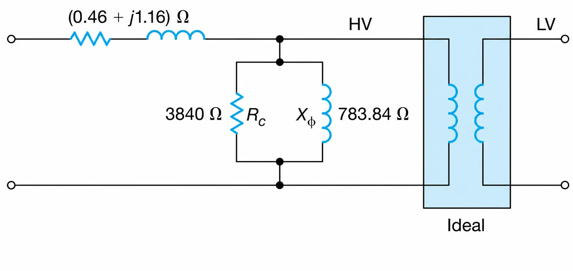
Figure 2-13 equivalent circuit referred to the HV winding
Waveform of Excitation Current
When one of the transformer’s windings is open-circuited while the other is connected to rated voltage, the resulting current represents a small percentage of the transformer’s rated current. This is due to the transformer’s high magnetization impedance and to the infinite impedance seen by one winding while the other is open-circuited. This current is referred to as the excitation current ($I_{exc}$). In practice,
$$I_{\text{exc}}=(3\%\rightarrow10\%)\,I_{\text{rated}} \ \ \ \ \ (2.26)$$
The theoretical derivation of the exciting current’s waveform is obtained from the transformer’s B-H characteristic as follows: Draw the waveform of the sinusoidal flux on an ωt-axis. Then, on the same coordinate system, draw the waveform of the exciting current. Refer to Figure. 2-14(a). The waveform of the flux can easily be obtained, because, it will be noted, the points $\left ( \alpha _{1},0 \right )$, $\left ( d_{1},d_{2} \right )$, and $\left ( g_{1},0 \right )$ are π/2 radians apart and correspond, respectively, to zero, maximum, and zero values of the flux. In other words, the critical points of the flux are known during half the period of its sinusoidal function. The resulting flux waveform is sketched in Figure. 2-14(b).
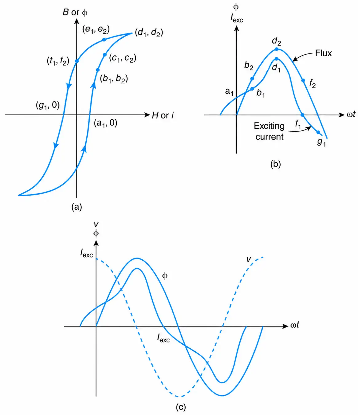
Figure 2-14 Typical magnetic characteristics of transformers. (a) B-H curve. (b) Instantaneous values of flux and exciting current. (c) Instantaneous values of induced voltage, flux, and exciting current.
The magnitude of the exciting current at each of the coordinate points $\left [ \left ( \alpha_{1},0 \right ),\left ( b_{1},b_{2} \right ),\left ( d_{1},d_{2} \right ), etc \right ]$ of the B-H curve is given by the abscissa of these points. This is shown in Figure. 2-14(b). The transformer’s voltage, flux, and exciting current are shown in Figure. 2-14(c).
The exciting current is not sinusoidal because of the nonlinearities of the B-H curve, and so a conventional phasor diagram of the exciting current cannot be drawn. However, its harmonics content, or its equivalent sinusoidal functions, can be found by using the Fourier series analysis. The Fourier series method is a mathematical tool used to determine the harmonic content of no sinusoidal waveforms.
It can be shown that the exciting current is made up of “odd harmonics,” that is, a fundamental term, a third harmonic, a fifth harmonic, and so on. The third harmonic can be as high as 40% of the fundamental term.
Components of Primary Current and Corresponding Fluxes
When a transformer is connected to its primary supply voltage while its secondary is open-circuited, it draws (as stated previously) a small percentage of its rated current ($I_{exc}$) . Although this current is small, it produces rated flux within the core of the transformer.
As soon as an impedance is connected to the transformer’s secondary (see Figure. 2-15(a)), a load current will flow. This current will produce the flux ($\phi_{2}$) that opposes the flux of the primary current. This cannot be tolerated because it would be accompanied by a reduction of the voltage induced in the primary $[v_i = -N \left(\frac{d\phi}{dt}\right)] $, which would result in violation of KVL $(V_1 = v_i)$. To overcome this opposition, the current drawn by the primary winding increases in such a way as to completely cancel the magnetic opposition of the secondary current.
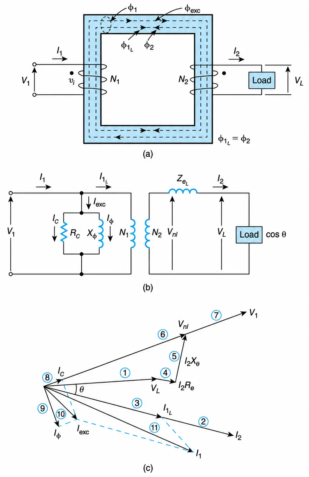
Figure 2-15. Transformer. (a) Polarity and component fluxes. (b) Equivalent circuit. (c) Phasor diagram.
The quantity of primary current needed to produce flux sufficient to completely neutralize the opposition of the secondary current is called the load component of the primary current. It is designated by $I_{1L}$. Alternatively, the mmf of the secondary winding ($N_{2}I_2$) is equal and opposite to the increase in the mmf of the primary winding ($N_{1}I_{1L}$). As a result, the effective mmf of the transformer at negligible leakage flux is $N_{1}I_{exc}$.
The increase in the primary current that accompanies the flow of current in the secondary could also be justified by considering the following principle of energy conservation:
$$\text{Energy drawn by the transformer} = \text{Energy delivered to the load} + \text{Energy consumed within the transformer}$$
The energy demand of the load is met by an increase in the magnitude of the primary current and its power factor relative to the no-load condition.
Under nominal operating conditions, the primary current is made up of two components. One, the exciting current, is required to magnetize the transformer; the other, its load component ($I_{1L}$) , is needed to cancel the opposition of the secondary current. In mathematical form, and as shown in Figure. 2-15(b),
$$I_1=I_{\text{exc}}+I_{1L} \ \ \ \ \ (2.27)$$
The primary current $I_{1}$ is almost sinusoidal because its nonsinusoidal component, the exciting current, is negligible in comparison to its sinusoidal load component.
The flux of the primary current is shown in Figure. 2-15(a). Its mathematical representation is
$$\phi_1=\phi_{\text{exc}}+\phi_{1L} \ \ \ \ \ (2.28)$$
where $\phi_{1L}$ is the load component of the primary flux.
Phasor Diagram
Refer to Figure. 2-15(b). The transformer delivers power to a lagging-power-factor load. The windings turns ratio and the load voltage $V_{L}$ normally are known. The load current $I_{2}$ is obtained from the load characteristics. The basic circuit equations are
$$V_1N_2=V_{nl}N_1 \ \ \ \ \ (2.29)$$
And
$$V_{nl}=V_L+I_2Z_{eL} \ \ \ \ \ (2.30)$$
These equations, together with Equation (2.27), are used to construct the phasor diagram shown in Figure. 2-15(c). The encircled numbers indicate the sequence of steps that you may follow in order to simplify its construction.