Instrument Transformers and Wiring Diagrams

This section discusses instrument transformers and wiring diagrams. Wiring diagrams illustrate how the instrument transformers are interconnected to the various measuring and indicating meters. These topics not only supplement the basic transformer concepts but also give an overview of the practicing engineer’s work.

Instrument Transformers

Instrument transformers are used to measure and control electrical parameters (voltage and currents). There are many different classes, each with a specific range of measuring accuracy.

Instrument transformers used for relaying and indicating purposes have a larger margin of error than those used for measuring the power and energy on which the billing demand of a particular plant is based.

There are two types of instrument transformers: potential transformers, used for measuring voltage, and current transformers, used for measuring current (see Figure 2-52). The equipment connected to their secondaries constitutes the so-called load, or burden. In normal operation, the burden of the current transformer is of very low impedance, while the load on the potential transformer is of very high impedance. An elementary representation of instrument transformers and some of the meters connected to their secondaries is shown in Figure 2-53.

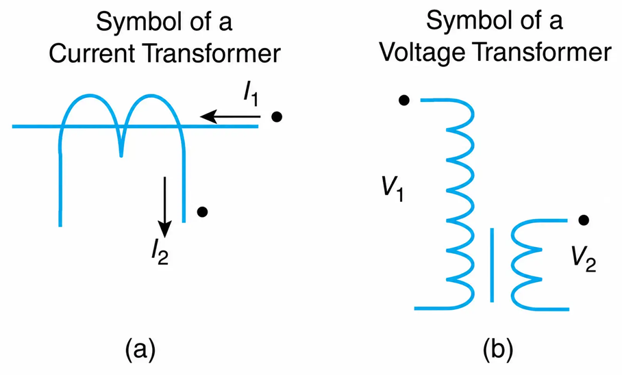
Figure 2-52 Symbols of instrument transformers. (a) Current transformer. (b) Voltage transformer.

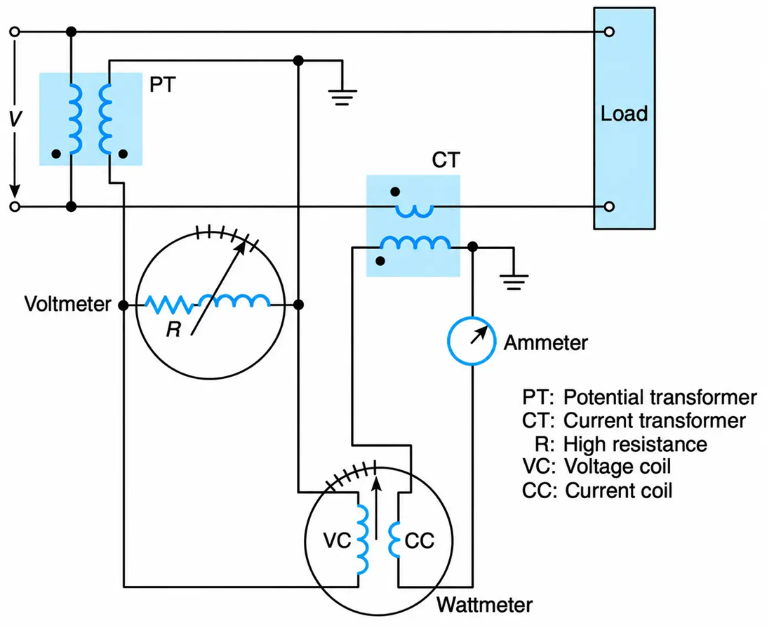
Figure 2-53 An elementary representation of instrument transformers and measuring meters.

The polarity and the grounding of the potential and current transformers are as shown in the Figure Correct polarity identification will lead to correct instrument connections; proper device grounding will ensure the safety of personnel and the protection of equipment.

Potential Transformers

Potential transformers are used for stepping down voltages to nonhazardous and conventional voltage levels—normally 120 volts—for measuring and controlling purposes.

As shown in Figure 2-54, their primary winding is connected in parallel to the high-voltage circuit whose voltage is to be measured. The voltage across the secondary winding is applied to potential coils of meters, relays, and other instruments, depending on what is desired.

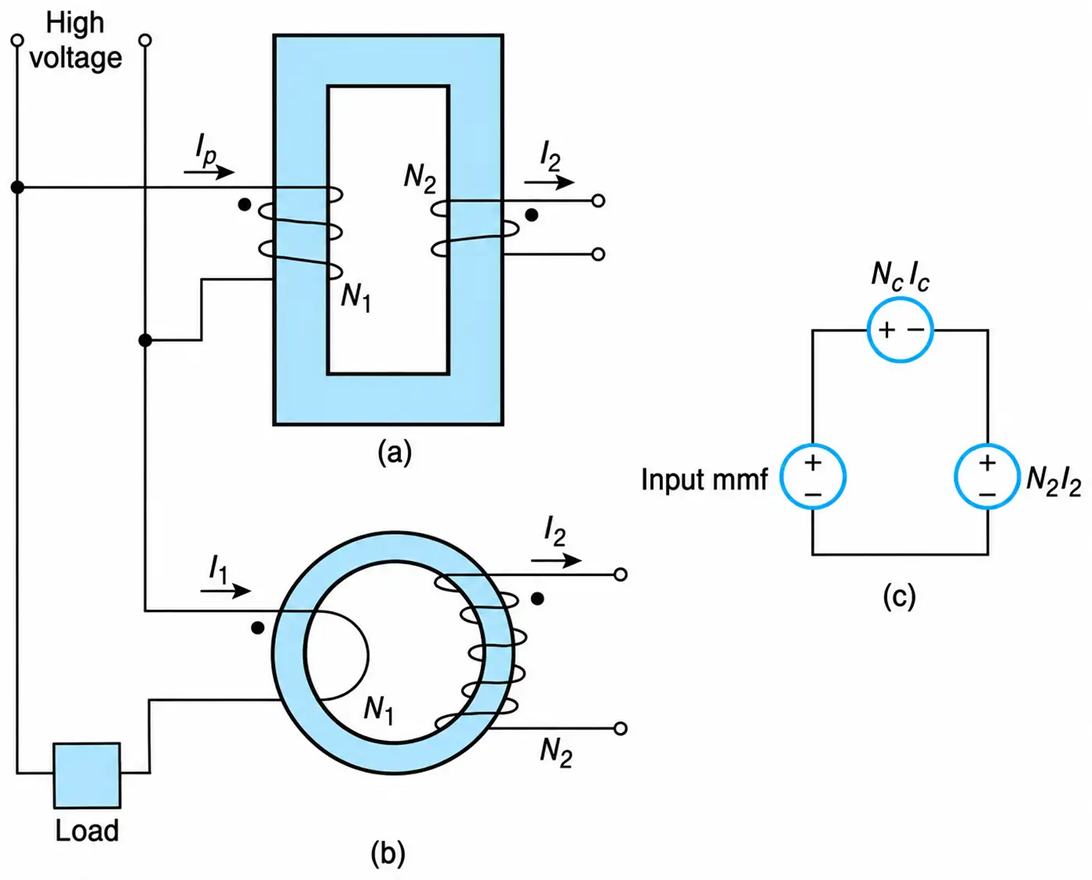
Figure 2-54 Instrument transformers. (a) Schematic diagram for a PT. (b) Schematic diagram for a CT. (c) Magnetic equivalent circuit for instrument transformers.

Refer to Figure 2-54(c). By applying KVL, we obtain

$$\text{input mmf} = N_c I_c + N_2 I_2 \ \ \ \ \ (2.65)$$

where ‍N_CI_C is the mmf within the material and on whose magnitude the magnetization level of the PT depends. For a PT, the above expression becomes

$$I_p N_1 = N_c I_c + N_2 I_2 \ \ \ \ \ (2.66)$$

Where I_P is the current through the PT’s primary winding. The magnitude of the primary voltage of a potential transformer is nearly constant; therefore, the magnitude of the flux within the magnetic material is also constant (see Equation (2.7)). For all practical purposes, this results in a constant-magnitude mmf within the material, regardless of the magnitude of the load current.

The variation of the PT’s magnetization level from a no-load (I₂ = 0) to a full-load operating condition is shown in Figure 2-55(a). The small change in the levels of magnetization (from no-load to full-load operating condition) is due to leakage flux that saturates part of the magnetic material.

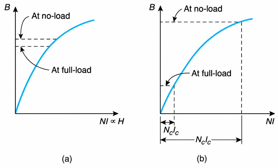
Figure 2-55 Levels of magnetization from no-load to full-load for instrument transformers. (a) Potential transformers. (b) Current transformer.

When a PT’s secondary winding is shorted, the resulting high current will produce high winding losses. Consequently, if the transformer is not properly protected, it will be damaged and may become a fire hazard.

Current Transformers

Current transformers step down the current of the primary circuit to conventional standard levels (normally 5 amperes) for measuring and controlling purposes. As shown in Figure 2-54(b), their primary is connected in series with the circuit whose current is to be measured. The current of the secondary winding is applied to current coils of meters and relays. Under normal operating conditions, the current through the load is constant, and thus the input mmf ‍N₁I₁ to a CT is also constant.

Rewriting KVL in the magnetic circuit of Figure 2-54(c), we have

$$\text{input mmf} = N_c I_c + N_2 I_2 \ \ \ \ \ (2.67)$$

The above expression for a CT becomes

$$N_1 I_1 = N_c I_c + N_2 I_2 \ \ \ \ \ (2.68)$$

From the last equation it becomes evident that a CT’s magnetizing mmf  varies from its maximum value at zero secondary current (open secondary) to its minimum value at maximum secondary current (shorted secondary). The variation of the CT’s magnetization level from the no-load to full-load operating condition is shown in Figure 2-55(b).

A low magnetic potential drop within the material corresponds to low levels of flux and core loss. For this reason, energized CT’s have their secondaries either shorted or connected to low impedance devices. When an energized CT has its secondary open-circuited, it will be damaged (a problem usually encountered in the commissioning of new plants) by excessive magnetic losses.

A CT hooked up to a live feeder should never have its secondary open-circuited. This would result in a higher level of magnetization, which in turn would induce a high potential across the secondary terminals. This will endanger working personnel and will destroy the CT (owing to excessive core loss).

For the purposes of comparison, the characteristics of CT’s and PT’s are summarized in Table 2-3.

Table 2-3 Main Characteristics of PT’s and CT’s

Exercise

When the single-phase load of Figure 2-54 is accidentally shorted, what will be the effect on the potential and current transformers?

Shorting the load will increase by many folds the current through the primary winding of the CT. As a result, the CT will be damaged—if no precaution is taken—due to excessive copper losses. The PT’s primary current will remain at its nominal level

Optical Instruments

Optical instrument transformers refer to potential and current transformers, which contrary to classical PT’s, measure the voltage and current to a distribution system without being in contact with the live conductors. They are very expensive and are presently used in high-voltage substations. Their usage, however, will be extended to lower voltages because of their great advantages, such as security of personnel, very low maintenance, high accuracy, no magnetic or copper losses, prevention of fires, no ferro resonance, and small size.

*In general, a light polarizing device, depending on its con Figure ration, transmits part of the light. This process of polarization can be easily observed at night when you use reading glasses and look at the street incandescent lights and/or when you look toward the lights of incoming cars when driving (Figure 2-56).

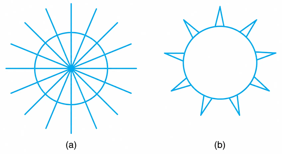
Figure 2-56 Light bulb. (a) Unpolarized light. (b) Light (polarized) as seen with reading glasses.

Optical Current Transformers

The optical CT consists of two sections, one of which produces opposite rotating circular polarized lights and the other incorporates light detecting diodes.

For a given wire to a distribution network, two circular polarized lights are generated (Figure 2-57), one of which is aided by the magnetic field of the conductor’s current $(\Phi \alpha I)$ and the other is opposed. The change in the illumination level is detected by the light-detecting diodes. The diode’s current is further processed, and the output of the optical sensor is transmitted to the control room by wireless technology or by optic fibers.

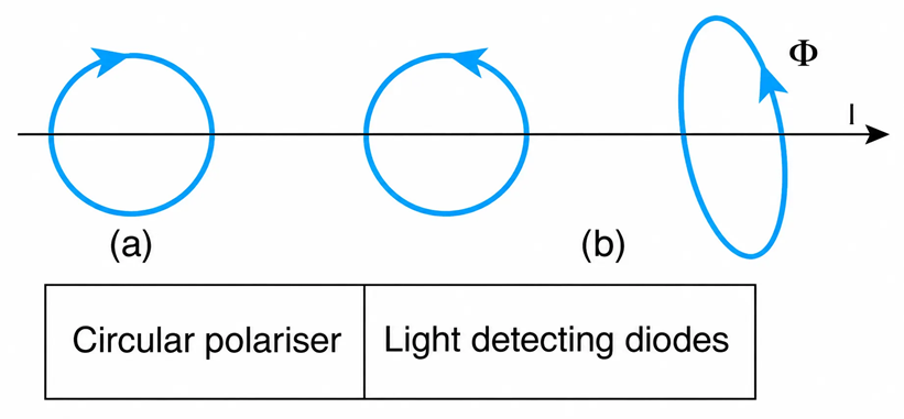
Figure 2-57 Schematic diagram of an optical CT. (a) Polarized circular light encircling a wire and magnetic field of cable’s current. (b) Generation and detection of polarized light.

PT’s

The sensor of an optical PT detects the intensity of the electric field (E) produced by the conductor’s current. The intensity depends on the distance of the sensor from the section of the wire and the voltage of the wire’s field.

The corresponding voltage produced ($v = -\int E\,dx$) is the weighted average of the output of the detecting elements.

Some manufacturers combine the optical CT’s and PT’s in the same unit.

Wiring Diagrams

Wiring diagrams are electrical drawings that use conventional symbols to indicate the actual hook-up of meters. The wiring diagram of a digital meter is shown in Figure 2-58. It measures many parameters such as voltage, current, power, power factor, and harmonics. Such units are equipped with a display and a set of push buttons. When a parameter is to be displayed, a corresponding push button is depressed. These meters can also send “measuring pulses” to computers, which in turn can print out the instantaneous variations of the system parameters.

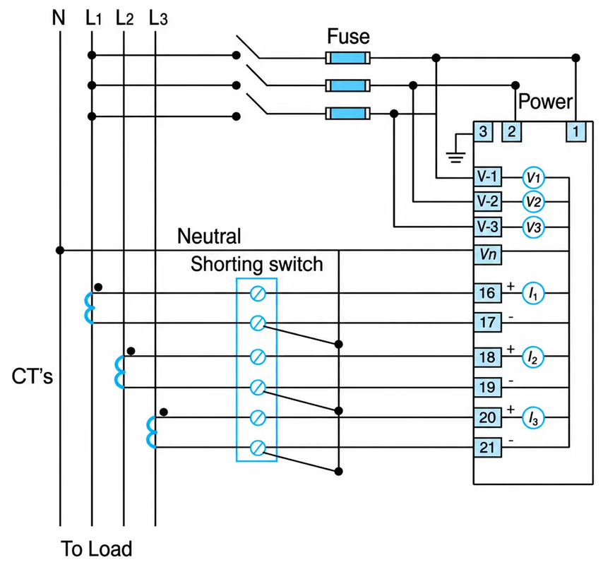
Figure 2-58 Wiring diagram of a digital multimeter.

Example 2-10

For the single-phase transformer shown in the one-line diagram in Figure 2-59, determine the ammeter reading for the following operating conditions:

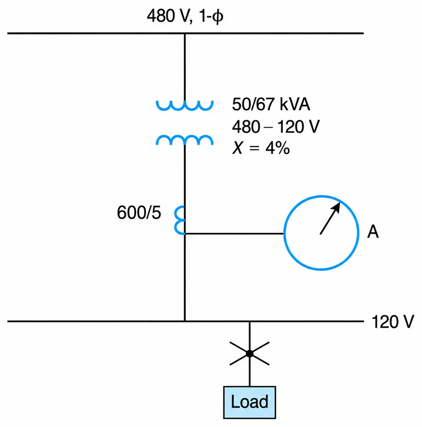
Figure 2-59 Single-Phase Transformer in One-Line Diagram

• The transformer delivers 80% of its base kVA at nominal voltage.
• The transformer delivers 100% of its fan-rated kVA.
• The transformer’s secondary feeder is shorted.

Solution

a. When the transformer delivers 80% of its rated kVA, the magnitude of the current in the line (or the ammeter reading) is

$$I = 0.8\left(\frac{50 \times 10^3}{120}\right) = 333.33\ \text{A}$$

The CT’s secondary current will be

$$I_{CT} = I_{\text{actual}} \times \text{turns ratio}$$

$$I_{CT} = 333.33\left(\frac{5}{600}\right) = 2.78\ \text{A}$$

This is also the current through the ammeter, but the ammeter is always calibrated to give the actual current through the load.

b.  Similarly, the ammeter reading will be

$$I = \left(\frac{67 \times 10^3}{120}\right) = 558.33\ \text{A}$$

The CT’s secondary current will be

$$I_{CT} = 558.33\left(\frac{5}{600}\right) = 4.65\ \text{A}$$

c. The impedance of the transformer depends on its base kVA and not on its fan-rated kVA. The kVA’s significance is that if the transformer windings are externally cooled, they can carry higher currents without becoming overheated. Since the applied voltage and the transformer impedance remain constant, the short-circuit current is independent of the level of operating kVA. Thus, the ammeter reading on short-circuit conditions is

$$I = \left(\frac{1}{0.04}\right)\left(\frac{50 \times 10^3}{120}\right) = 10.42\ \text{kA}$$

The current through the CT’s secondary winding will be

$$I = 10.42 \times 10^3 \left(\frac{5}{600}\right) = 86.81\ \text{A}$$

a. Refer to Figure 2-59. When the ammeter reads 1500 A and has an accuracy of 99%, what is the apparent power drawn by the inductive load?

b. What is the power factor of the load when the kW meter reads 2000 kW and the reactive power meter reads 1500 kVAR?

Solution

a. The scales on switchboard-type meters are calibrated in terms of the line-side parameters. Thus, the current through the 4.16 kV lines is

$$I_L = \frac{1}{0.99}(1500) = 1515.15\ \text{A}$$

By definition, the apparent power is

$$|S| = \sqrt{3}\,V_{L-L} I_L = \sqrt{3}(4.16)(1515.15) = 10{,}917.17\ \text{kVA}$$

b. The real and reactive powers are given, respectively, by

‍‍$$P = \sqrt{3}\,V_{L-L} I_L \cos\theta$$

$$Q = \sqrt{3}\,V_{L-L} I_L \sin\theta$$

Thus,

$$\theta = \arctan\frac{Q}{P} = \arctan\frac{1500}{2000} = 36.9^\circ$$

The power factor is

$$\cos 36.9^\circ = 0.80\ \text{lagging}$$

Ferroresonance

Human Resonance

Resonance in general is a condition that results in maximum response (love, hate, indifference, and so forth). Some people instinctively love red colors, while others hate them or yet some others are indifferent to them. The future of an individual most likely will be strongly influenced by his or her inner inclination (resonance) in conjunction with that of fellow humans (boss, partner, friend, and such). It has been reported that an international bank, in order to select the most suitable employees to a managerial position, subjects all candidates to a questionnaire (searching for resonance) and from this, a decision is made that is apparently 100% accurate.

Linear Resonance

In the linear resonance, the overvoltages and overcurrents are of predictable magnitude. Such a resonance takes place when the circuit’s inductive reactance is equal to the capacitive reactance. Furthermore, the circuit’s power factor is equal to 100%, and the magnitude of the resulting overvoltages and overcurrents are sinusoidal and of predicable frequency. Similarly, a building is characterized with linear resonance whose frequency is in the range of 4–6 Hz.

Nonlinear Resonance

In nonlinear resonance the voltages and current are very high and of unpredictable frequency. The nonlinear resonance is known as a ferroresonance. It was observed almost 100 years ago that ferroresonance was taking place in distribution systems whose transformers were made from ferrous materials (iron laminations).

Ferroresonance depends on the circuit’s initial conditions, the applied voltage, the nonlinear circuit inductance, and on the capacitance between cables and/or cables and ground. In ungrounded systems, the voltages developed could be up to 4 pu, while in the grounded systems, voltages could reach 2.5 pu.

The inductance is inversely proportional to the permeability, which in turn is the slope of the material’s B-H diagram. At higher than nominal voltages, the transformer is driven into saturation, the permeability is reduced, and thus the inductance is increased.

Many causes can initiate ferroresonance, but the main one is the variable inductive reactance of the power, potential, and measuring potential transformers that are driven into saturation. The initiation of this phenomenon could be attributed to the lightning strokes, breaker switching, or malfunctioning and single-phase operation of a three-phase distribution system.

One way to mitigate the effects of resonance is to oversize the transformers so that an accidental increase in the supply voltage will not drive them into saturation and/or add a resistance (damping effect) on the secondary windings of the transformers.

It has been well publicized that if a small step-down PT and a small capacitor in a control system initiated ferroresonance, that can cause the failure (insulation damage) of dozens of downstream motors.

K-Factor of Transformers

A transformer designated as k-type (k-4, k-9, k-13, etc.) indicates that it will not be overheated when the k-factor of the line currents is lower than that of the transformer.

When k=1, it means that the transformer will not be overheated when it supplies rated power to linear load—that is, when the load does not draw any harmonic current. The rate of heat loss within the transformer is the sum of the core loss (eddy-current and hysteresis loss) plus the stray losses and I²R of its windings.

The eddy-current losses and hysteresis losses are nonlinear functions of the currents’ frequency.

By far, the largest effects of the harmonic components of the currents are on the eddy-current losses.

Calculation of the K-Factor

The k-factor is defined as follows:

$$k = \sum_{h=1}^{h_{\max}} I_h^2 h^2 \ \ \ \ \ (2.69)$$

where h stands for the number of the harmonic and I_h is the rms current of harmonic h, in per unit of the line current.

Example 2-12

The line current $(\iota)$ in a power distribution system is

$$\iota = 10\sin\omega t + 4\sin 3\omega t + 2\sin 5\omega t + \ldots$$

Determine the k-factor.

Solution

The rms value (I) of the line current is

$$I = \sqrt{\left(\frac{10}{\sqrt{2}}\right)^2 + \left(\frac{4}{\sqrt{2}}\right)^2 + \left(\frac{2}{\sqrt{2}}\right)^2} = 7.746\ \text{A}$$

and the per-unit values of the current components are

$$I_1 = \left(\frac{10/\sqrt{2}}{7.746}\right) = 0.9129$$

$$I_3 = \left(\frac{4/\sqrt{2}}{7.746}\right) = 0.3651\ \text{pu}$$

And,

$$I_5 = \left(\frac{2/\sqrt{2}}{7.746}\right) = 0.1826\ \text{pu}$$

From Equation (2.69), we obtain

$$k = \left[(0.9129)(1)\right]^2 + \left[(0.3651)(3)\right]^2 + \left[(0.1827)(5)\right]^2 = 2.8664$$